Worksheet 2: The Tipping Curve
Refer to Ch2 of the ERA Notes.
Recall that if the zenith opacity is sufficiently small, we can write the system temperature of a telescope as follows:
$T_\mathrm{sys} = (T_\mathrm{r} + T_\mathrm{cmb})+T_\mathrm{b}$
where $T_b$, the equivalent temperature of the atmosphere, is given by $T_b=T_{atm} \tau_z \sec z$.
Since $T_r$ and $T_{cmb}$ are constants, we can thus write down the following expression for the tipping curve:
$\tau_z \approx \frac{\Delta T_{sys} / T_{atm}}{\Delta \sec z}$
Questions
- For each data set (measurement), use the data provided to estimate the system temperature and calculate the temperature of the CMB.
- For each measurement, calculate the RMS deviation of the receiver temperature $T_\mathrm{r}$. Now, plot the RMS deviations and the measured temperature and the calculated temperature $T_\mathrm{cmb}$. What can you conclude?
Tips & Assumptions
- You may assume that the ambient atmospheric temperature ahs been measured to be $T_\mathrm{atm}=300K$.
- I have used a simple python library to fit a straight line to the tipping curve. This is a generic library to fit polynomials to data, and there is an associated function to calculate the resulting coefficients.
- The slope of the tipping curve is $[T_\mathrm{r}+T_\mathrm{cmb}]/T_\mathrm{atm}$, and the x-intercept is $\sec(z)$. Since the data is noisy, you can use a fit to estimate these parameters.
- The $T_\mathrm{r}$ receiver measurements resemble a Gaussian distribution. You can use this concept to estimate the mean value $<T_\mathrm{r}>$, and the RMS deviation of the measurements.
Loading and Plotting the Data
The tipping curves are all located in the directory /data/ast2003h/.
You will find the following files in there:
- tipping-curve-1.txt
- tipping-curve-2.txt
- tipping-curve-3.txt
- tipping-curve-4.txt
- tipping-curve-5.txt
- tipping-curve-example.txt
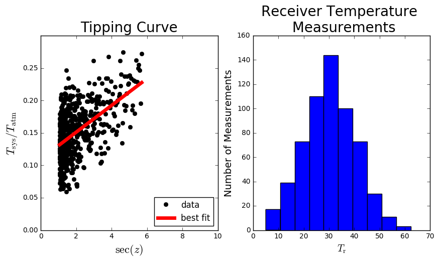
In each file, column-1 corresponds to $\sec(z)$, column-2 corresponds to $T_\mathrm{sys}/T_\mathrm{atm}$ and column-3 corresponds to measurements of $T_\mathrm{r}$.
Note: In tipping-curve-example.txt there is an extra column-4, which corresponds to a fit to the tipping curve data. This is not present in the other files.
In the cells below I illustrate how to extract the data from tipping-curve-example.txt, and I plot the relevant data in two subplots. I’ve also plotted the best fit curve that I calculated previously.
import numpy as np
import pylab as pl
%matplotlib inline
data = pl.loadtxt('/data/ast2003h/tipping-curve-example.txt')
secz = data[:,0]
tsys_over_tatm = data[:,1]
trx = data[:,2]
fit = data[:,3]
pl.figure(figsize=(10,5))
pl.subplot(121)
pl.plot(secz, tsys_over_tatm, 'ko', label='data')
pl.plot(secz, fit, 'r-', lw=5, label='best fit')
# This sets up the x/y limits, axis labels and plot title.
pl.xlim(0,10)
pl.ylim(0,0.3)
pl.xlabel('$\sec(z)$', fontsize=16)
pl.ylabel('$T_\mathrm{sys}/T_\mathrm{atm}$', fontsize=16)
pl.legend(loc=4, numpoints=1)
pl.title('Tipping Curve', fontsize=20)

pl.subplot(122)
pl.hist(trx)
pl.xlabel('$T_\mathrm{r}$', fontsize=14)
pl.ylabel('Number of Measurements', fontsize=14)
pl.title('Receiver Temperature \n Measurements', fontsize=20)
<matplotlib.text.Text at 0x7f168281b0d0>
Enter your code below.
Remember to include your name and your student number.