Designing an Interferometer Array

In this group project, your team will be designing a radio antenna array (an interferometer). You will need to balance a variety of technical and scientific constraints, and you will use a variety of tools to design candidate arrays, simulate the operation and quantify the performance.

Your telescope will be built to conduct a single survey for its operational lifetime, and the target sensitivity of your survey is \(\sigma_\mathrm{survey}=10\mu\,\mathrm{Jy}\).

Introduction

An ideal radio interferometer measures the Fourier transform of the brightness distribution from an astronomical source. In practice, the convolution of the telescope’s sampling function and the source’s brightness distribution is measured. Image reconstruction is the process of undoing this convolution (or the Fourier multiplication), and is often referred to as deconvolution.

The telescope’s sampling function plays a central role in image reconstruction – you need as many independent measurements as possible to reconstruct an image, but redundant measurements also help with calibrating a radio telescope. The resolution of your telescope is determined by the longest baseline, so the longer the baseline, the better the resolution. You will find, however, that having a single (or a few) long baselines is not sufficient to ensure good resolution – you need many long baselines, and you need many intermediate baselines to provide good sampling of the Fourier domain. Finally, while higher resolution is a good thing, you need short baselines to observe extended sources (e.g., gas around nearby galaxies).

Therefore, the design of a radio array is a fine balance between resolution and sensitivity. Resolution motivates for long baseline, and sensitivity motivates for more antennas.

Your Project

Your objective is to design a radio interferometer. Your design will be constrained by scientific, budgetary and technical considerations, so take note of the factors mentioned here. You will submit your report as a scientific paper, and your team will present your findings at the project conference. This is a research project, so please try to find important/relevant references where possible.

Groups

Each group will comprise 4 students, and it is expected that each student makes an equal contribution to the project. Each group must nominate a group secretary, who will report on the progress of the group. The secretary will take the responsibility of arranging group meetings, and will represent the group’s concerns and best interests.

Please watch the Vula site for more information on each group.

What to Submit and Important Dates

• Friday, 3 November 2017: Submit your final configuration in a text file, and an advanced draft of your report in PDF format.
  • We will evaluate the performance of your configuration, and review your report for questions and comments that will be addressed at the presentation.
• Wednesday, 8 November 2017: Your team will present a 20-minute presentation (powerpoint/keynote). Each member will have to present for 5-minutes. This will be followed by a 5-minute Q&A session.
• Friday, 10 November 2017: Submit the final version of your report in PDF format.

Constraints

Your team has a budget of 200,000,000 credits (CR) to design an optimal antenna layout, and a daily operational budget of 2,000,000CR. That is, once you have constructed your telescope, you will have 2M-CR/day to operate your telescope. The following constraints apply:

• You have 5-years to build and operation your telescope.
• Each dish costs 100,000CR to build.
• You will need some cable and infrastructure for each dish. For each dish, this infrastructural cost is 1000CR per metre away from the centre of the array. For example, the infrastructural cost for a dish that is 3200-metres away from the centre of the array is 3,200,000CR.
• The maximum baseline cannot exceed 20km.
• The dish size is 12-metres. Therefore, the minimum distance between each dish is 12-metres. In practice, the real distance is slightly larger to avoid shadowing.
• Deduce/invent a way to measure how well your radio array has reconstructed the test image, which is a measure of image fidelity. For example, the difference between the output image (i.e., after imaging) and your original test image ought to be as small as possible. Another possible metric could be the ratio of the test and output images; perfect reconstruction would produce a ratio-image that is unity everywhere. In practice, neither metric will be perfect. There is, however, a task in CASA that will do an evaluation for you, and will calculate a fidelity image for you. Consult the guide on simulating observations for more details and ideas.

Supplementary Material

I have provided a Jupyter Notebook that contains information and supplementary material for the following constraints:

• Operational costs: The daily operational costs of a telescope are not constant as a function of time. In your project I have included a very simple relation on how the operational costs scale as a function of time.
• Which \(T_\mathrm{sys}\) value to use for your array, based on how many antennas you end up building. Providing cryogenic cooling for a large dish array is expensive business. While you can achieve a desirably low system temperature for a modest number of dishes, you will soon run out of funding if you start cooling a large number of dishes. Therefore, while it may be a good idea to build a huge numbr of dishes, you may not be able to cool them sufficiently to achieve a good sensitivity.
• Antenna efficiency as a function of build time. The build time for a dish varies from 0.5-2 days, with a 12-hour build time yielding antennas with the lowest efficiency, and a 2-day build time producing dishes with a 100% efficiency. This is a soft limit on the number of dishes that you can produce.
• How to calculate the sensitivity of your telescope for a given \(T_\mathrm{sys}\) using the radiometer equation.
  • You will not be able to simulate the full observations of your survey (e.g., thousands of hours), neither will it be feasible to create a suitably deep mock image (e.g., thousands of sources). Your simulation will be of a single day’s worth of observations. Depending on your design and your parameters, you can calculate the sensitivity of your telescope, and therefore construct a mock-image where the faintest sources are a few multiples of the sensitivity.

Science and Sensitivity

Your telescope will be built to conduct a single large radio survey. You will need to finish this survey before the end of the 5-year lifetime of your telescope. The target sensitivity of this survey is \(\sigma_\mathrm{survey}=10\mu\,\mathrm{Jy}\).

Since you are only observing a single channel, the sensitivity of your radio telescope is given by the simple equation:

where \(\eta\) is the efficiency of your telescope, \(\nu=10\,\mathrm{MHz}\) is the bandwidth of your single channel, and \(k_\mathrm{B}=1.38\times10^{3}\,\mathrm{Jy\,K^{-1}}{}\) is the scaled Boltzmann constant.

The aim of your telescope is to achieve the target sensitivity. You will need to balance the system temperature, number of dishes, efficiency and total observational time to achieve this target sensitivity.

\(\sigma_\mathrm{survey}\) is a measure of the faintest source that you can measure with any degree of confidence with your radio telescope. In practice, a multiple of this value is used as the threshold for source identification, e.g., a \(3\sigma_\mathrm{survey}\) source.

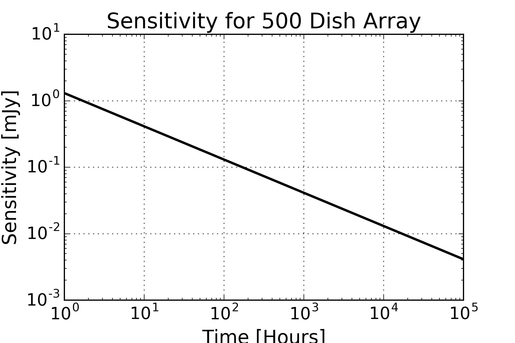
In the image below I illustrate the typical sensitivity as a function of time, for an array of 500-dishes, assuming perfect efficiency.

Remember that you need to state the time taken for your array to reach the target sensitivity, and create a sky-model where the faintest source are a few multiples of the per-day sensitivity.

Please make note of the following important points for your project:

• Your telescope will be placed at the de-facto central position of the MeerKAT array. You achieve this by specifying “MeerKAT” in the header of your antenna file.
• The operational frequency of your telescope is 1.420-GHz.
• Your telescope will only be observing a single channel of 10-MHz.
• The dummy-settings.txt file that I have provided set’s up observations for 2-hours/7200-seconds, with each integration being 10-seconds. Your integration time depends on the maximum baseline length! You can calculate this by looking at Section 3.1. of the Essential Radio Astronomy course.

You will be using simulations to evaluate the imaging performance of your telescope. However, it is unfeasible to calculate a simulation for the full duration of your observation (e.g., 2-years ~ 20,000-hours). Therefore, to evaluate the performance of your telescope, for a given \(N\), \(T_\mathrm{sys}\) and \(\eta\) you can calculate the expected sensitivity for the typical daily operational time \(\sigma_\mathrm{operational}\), e.g., 8-hours.

\(\sigma_\mathrm{operational}\) is an important number to keep in mind; the faintest sources in your mock image ought to be a few multiples of \(\sigma_\mathrm{operational}\).

Your Toolkit

All the software you require is available on the https://arcade-jupyter-hub.arc.ac.za virtual machine. You can download the scripts from this website (right-click save-as), or you can access it on the ARCADE machine in the following path/folder:

/data/ast2003h/project/2017-10-17/

I will add more scripts/resources in the /data/ast2003h/project/ path when necessary.

For this project, you will use the full suite of tools provided by Jupyter:

• The Jupyter Notebook (Python 2).
  • For visualising your uv and image data.
  • Creating array designs.
• The Terminal.
  • Running CASA.
  • Finding/accessing your data.
• The File Browser.
  • Changing the settings file(s).
  • Looking at plots (if you export them).
  • Writing your own scripts.

The flowchart below illustrates a possible method for you to generate your test images, antenna configurations and to evaluate the antenna array.

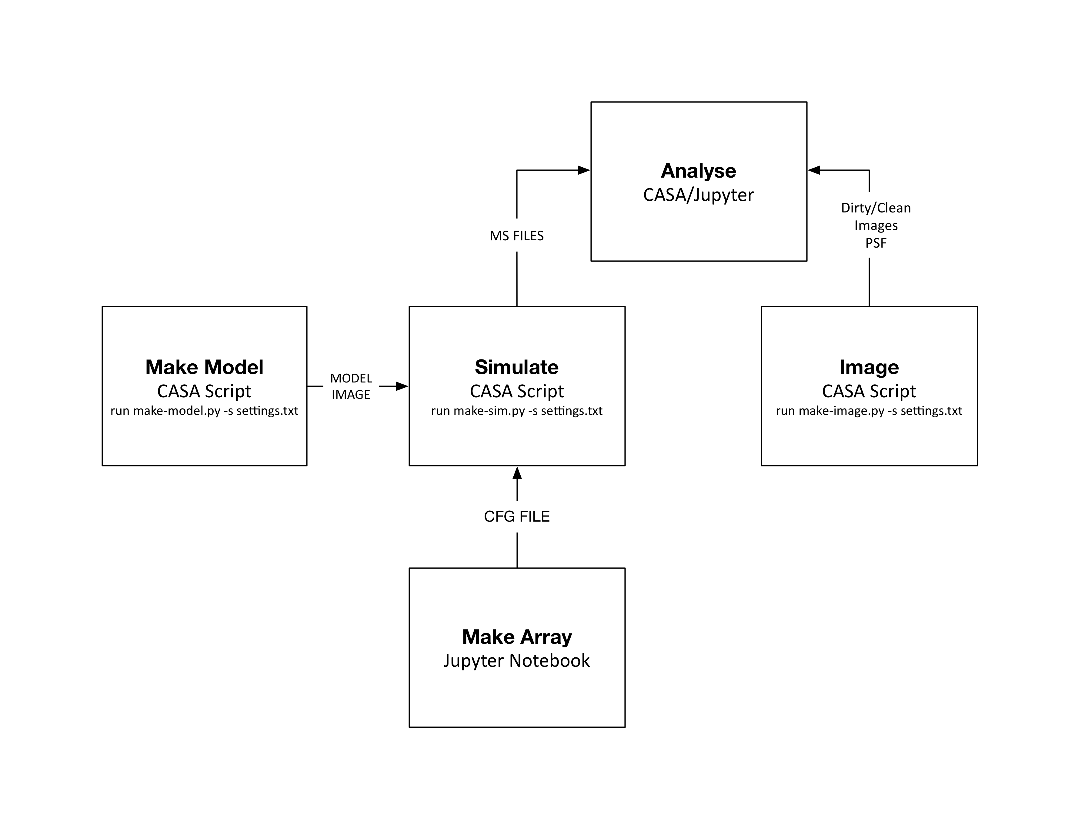
I have provided a few scripts and notebooks that will help with the simulation, imaging and analysis.

• dummy-settings.txt
  • This is a settings file that is used by each of the CASA scripts that I have provided.
• make_model.py
  • This CASA script creates a component list and constructs a model image, based on the source parameters in dummy-settings.txt.
• make_sim.py
  • Uses the CASA task simobserve to create a simulated measurement set. It creates a pointing file with a single pointing at the centre of your model, and creates the visibility data according to your observational setup, e.g., total time, number of integrations, etc…
• make_image.py
  • Uses the CASA task clean to image your simulated measurement. Remember that niters=0 makes a dirty image, which is the equivalent of an FFT, and niters>0 will clean the image, i.e., do deconvolution for niter loops.
  • Also uses exportfits, which exports a CASA image (a table) into a fits file.
• meerkat.cfg
  • A text file specifying the location of the MeerKAT antennas. Your array designs will have to be placed in a similar file for simulations.
• my-arrays.ipynb
  • An IPython notebook that imports and displays the MeerKAT positions, and illustrates how to make your own array configuration.
• plotting-image-data.ipynb
  • Uses APLPY to plot the fits files.
• plotting-uv-data.ipynb
  • Uses a package called pyrap and a customized languaged called TaQL to read the contents of a measurement set. I have illustrated how to plot a few important quantities.
• supporting-information.ipynb
  • This important notebook outlines the constraints of your pipeline.
• Source-distribution-per-sq-deg.ipynb
  • This notebook describes recommendations on how to make an astronomical sky model based on the NVSS. Please keep in mind that this is just an approximation to produce a reasonably realistic, and describes how to make a source image with a few tens of sources. In reality, the micro-Jansky radio sky has thousands of sources, but it is neither feasible nor necessary to simulate such a mock image.

The notebooks can be imported directly into your Jupyter Hub. The scripts, once they are in a suitable directory, can be executed as follows, for example:

• You have to run CASA from within a terminal:

    casa --nologger --log2term --nogui
  

• You can then run your script as follows:

    run make_model.py -s dummy-settings.txt
  

CASA

CASA stands for Common Astronomy Software Applications, and is a C++/Python package designed by the NRAO to do calibration and imaging for radio interferometric imaging.

CASA is an object-oriented descendent of the classical NRAO software AIPS, and is written in C++, with a (I)Python binding. You interact with and control the software using the IPython interface, but the underlying software is compiled C++ code.

Each of the scripts that I have provided make use of CASA tasks, and you can use these tasks directly, without the scripts.

• You have to run CASA from within a terminal:

    casa --nologger --log2term --nogui
  

• To look at the current and required inputs of a task, clean, for example:

    inp clean
  

• To get help on a task:

    clean?
  

• To set parameters:

    niters=1000
  

• Whenever you run a task, either via a script or directly, a .last file will be created. For example, if you run the script make_image.py, a clean.last file will be created which contains the last values used for clean. You can import those values into your current session as follows:

  tget clean
  

  or

  execfile('clean.last')
  

• Finally, if you choose to run CASA tasks yourself, you can save the commands/variables as follows:

  saveinputs(clean, 'clean.saved')
  

  You can retrieve the values from clean.saved by using execfile('clean.last').

Please adhere to scientific best practices when writing your report. Use a suitable typesetting software (e.g., LaTeX), and provide references to important literature.

Consultation and Further Information

I will be available for consultation on most Thursday and Fridays, during the usual AST2003H lecture slot.