Fourier Transform

Worksheet 1 focuses on using Python tasks to calculate the Fourier Transform of a few window functions. In this notebook, I will illustrate how you can generate a window function, and how you can calculate the associated Fourier Transform.

The Fourier Transform can be examined in many ways. The simplest interpretation is that the FT is a harmonic decomposition of a signal. You can calculate the FT analytically, if you’re lucky. If you’re even luckier, a finite Fourier Series will give you an accurate representation of your signal – provided that you have a simple signal. There is often an implicit assumption when calculating the analytical representation – that your input function goes from -infinity to +infinity.

In practice, astronomical signals are not perfect, simple sine-waves. Neither are they perfectly sampled, or sampled for infinite time. When you have a regularly sampled series, e.g., a time series, you can compute the Fourier Transform using the Fast Fourier Transform (FFT) Algorithm. This is what we’re doing in this worksheet – we are computing the FFT for a series of functions, and we are studying how similar or different the FT is to what we expect from the illustrations on the worksheet.

When in doubt, Google

There’s a reason why WS1 is short on details – there is a huge amount of resources on the internet that focuses on computing Fourier Transforms using python. In fact, if you Google Python Fourier Transform, the first hit will probably be the relevant SCIPY page.

Please note that there are lots of resources on how to generate window functions, such as the boxcar function. You can use a similar method to the one I’ve done below, or you can simply use a python function to define this. I leave it to you to figure it out.

Getting started

First, I’m going to import the important libraries, as suggested in the aforementioned URL. Note that %matplotlib inline command allows us to render plots within this notebook.

Also note how I have defined pylab and numpy in the Python namespace. This makes it easy to reference plotting and analytical functions from those libraries.

import numpy.fft as fft
import pylab as pl
import numpy as np
%matplotlib inline

The Shah Function

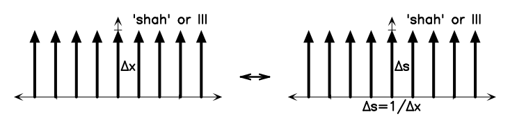
The Shah function (Comb) is a series of delta functions with some spacing dx.

The image below is from your WS1, and is one of the examples found in the ERA appendix on Fourier Transforms:

In the next cell I define the Shah function, by hand. Note how I use the np.mod function. This returns the remainder of division, so I’ve inserted an if statement that appends a 1 to the array if the index i is divisible by dx, and 0 if it isn’t. There are certainly many more methods to do this, but let’s do it the hard way for now.

I’ve also included comments on how I’ve constructed the Shah function and the associated plot.

# This is the step in the x direction.
dx = 10 
# Nx defines how many samples. The for-loop generates twice the number
# of samples defined in Nx.
Nx = 100

# Define empty arrays for x and y
x = []
y = []

# The for-loop runs from -Nx to +Nx in steps of 1.
for i in range(-Nx,Nx+1):
    x.append(i)
    # The if statement appends a 1 if (i,5)=0, and 0 if (i,5)!=0.
    if np.mod(np.abs(i), dx)<1:
        y.append(1.)
    else:
        y.append(0.)

# Python likes to do math on arrays, so I'm going to covert x and y.
x = np.array(x)
# Now y contains the Shah function, which I'll plot shortly.
y = np.array(y)
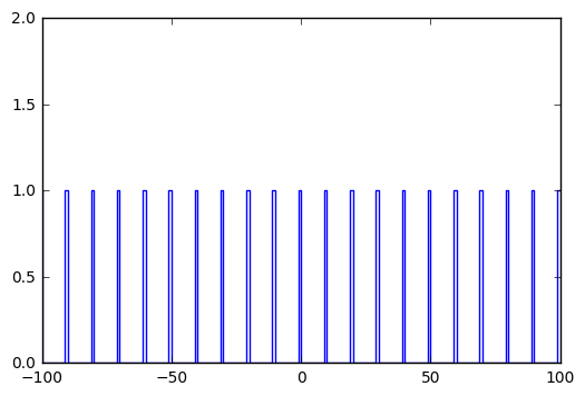
# Note that I'm using the step plotting function.
pl.step(x, y)
# Set the y-limits on the plot.
pl.ylim(0,2)

Calculating the Fourier Transform

Now that we have generated the Shah function, we can use the fft library defined above.

# I want the FFT to be smooth and well sampled, so I'm going to define 
# a variable that sets the number of points for the FFT.
nftpoints = 100

# Now, I can calculate the FFT of y.
# using norm='ortho' will normalize the FFT, and n=nftpoints will make 
# the FFT return the FT sampled with nftpoints.
F = fft.fft(y, norm='ortho', n=nftpoints)


# There is a method to calculate the associated frequency
# in the Fourier domain. 
# Now I'm going to include a fairly complicated command. 
# fft.fftfreq computes the frequency spacing, and fft.fftshift 
# shifts/sorts the frequency axis so that it plots nicely.
# The important command is fftfreq. 
freq = fft.fftshift(fft.fftfreq(nftpoints))

Plotting the FFT

Now that I’ve generated the window function and the associated FT, I can finally plot them in a way similar to the NRAO plot.

Here the subplot, step and ylim commands are important.

# First, plot the Shah function. 
pl.subplot(121)
# Plot this in a black line, this is what 'k-' is for.
pl.step(x, y, 'k-')
# Set the y-limit so that it looks pretty.
pl.ylim(0,2)
pl.title('Shah Function')


# Now, plot the FT.
pl.subplot(122)
# Note that I am plotting the absolute value of F, since F is an 
# array of complex numbers.
pl.step(freq, np.absolute(F), 'k-')
# Set the y-limit.
pl.ylim(0,2)
pl.title('FT of Shah Function')

<matplotlib.text.Text at 0x7ff2673bfc50>

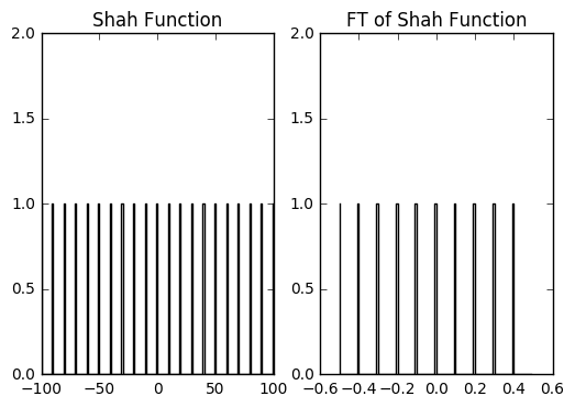
We need to note something important here. Recall that I set dx when I defined the Shah function above. Now, from the NRAO plot, I know that space between the spikes in the Fourier domain is given by the following: ds = 1/dx. You will note that this is the case in the plot above.